dynamical systems studies *interesting* behaviors in systems. one such class of interesting behaviors is equilibria, with stable and unstable varieties. but there’s more. consider a slight variation on the shaken inverted pendulum, where the shaking is happening horizontally. this leads to interesting and varied behaviors, depending (somewhat sensitively) on the initial conditions. some are *periodic* (they repeat over time); others seem to keep evolving and keep getting more & more complex. what is happening? how do we make sense of such? oh, there’s much more to learn about dynamical systems…
equilibria: stable & unstable
dynamical systems begins with the notion of equilibria — states that remain constant over time. In the simplest cases, one distinguishes between stable and unstable equilibria, though to specify what exactly these mean requires care (and math).
one simple example of stable and unstable equilibria is found in a rigid-rod pendulum, rotating about a pivot point (with or, as here, without, friction). letting the system evolve from a variety of initial conditions reveals a stable equilibrium (bottom) and an unstable equilibrium (top).
there’s a lot to discuss about this system. skipping ahead (for the sake of seeing something wonderful), let’s consider what happens when you give this system a shake, vibrating the pivot point up & down. the simulation indicates that past a criticla threshold of amplitude/frequency, shaking the pendulum converts the unstable equilibrium to a stable equilibrium.
that’s swell. but does the mathematics prove that this is the expected behavior? well, that’s one of the reasons why you take a dynamical systems course.
applied dynamical systems
in anticipation of teaching introductory dynamical systems & bifurcations to engineering students at penn this fall, i’m going to chat off and on about visualizing and (more importantly) simulating dynamical systems. this has challenged me in terms of my programming skills, but it’s a lot of fun to see theorems work in simulated systems.

vector fields & grid sampling
one of the most vexing things for me to illustrate is a planar vector field, especially when there is a singularity. there are so many distractions that arise from the canonical square-grid sampling that is endemic to software. here is an example with the linear vector field dx/dt = x ; dy/dt = -y

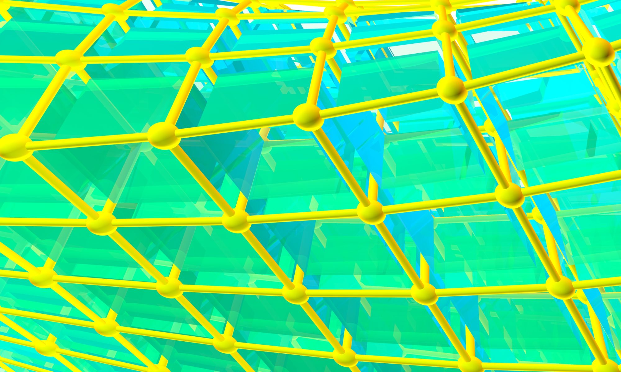
now for something completely different: the loxodromic grid, obtained by intersecting two circle’s worth of counterspinning spirals. you see these in sunflowers, pinecones, and the like. it seems as though nobody uses the term loxodromic grid (why was it in my head when i wanted to call this something? why did i know to use 137.5 degrees? intuition is a frustrating thing…). it also seems as though nobody ever plots vector fields on such a grid. pity, since that meant it took me a long time to figure out how to do it. but: it is worth the trouble…
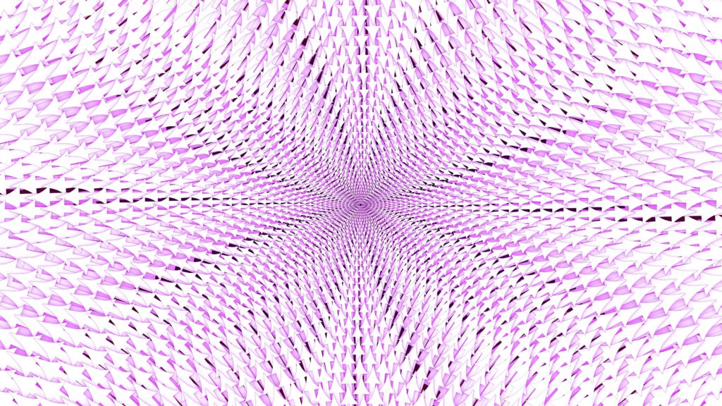
i really like the fact that the sampling gets increasingly tight near the equilibrium. i am simultaneously disturbed and pleased that the stable and unstable manifolds are “hidden” (as it were). it is fitting that you have a hard time visually getting on and staying on the stable manifold, since that’s exactly what happens in the flow. even the visual artefacts are instructive: note that near the origin, the tiny vectors are packed in such a way as to suggest not a circle (where the sampling points are) but a squashed ellipse. this is right: the flow squeezes and stretches areas.
this is not a perfect plot. but it is satisfying to me, after having tried and failed to make square and hex grids not look awful.
we now return to our scheduled program…
it’s been awhile since i’ve maintained this site or posted new content: the consequence of having no followers to disappoint! now that volume 4 of calculus BLUE (the hardest one by far) is done, i can go back to musing about illustration some more.
